Bell's polynomials, a topic typically reserved for advanced mathematics, have wide applications in fields ranging from combinatorics to physics. If you’ve encountered these intriguing polynomials but are unsure how they work or why they matter, you're in the right place.
This post explains Bell's polynomials in simple terms, breaking down their structure, significance, and applications. By the end, you'll have a strong understanding of what Bell's polynomials are, how they work, and why they are essential in mathematics.
What Are Bell's Polynomials?
Bell's polynomials, named after mathematician Eric Temple Bell, are sequences of polynomials that arise in combinatorics. They help us understand how to distribute objects into groups or derive more complex functions for mathematical analysis.
There are two major types of Bell's polynomials:
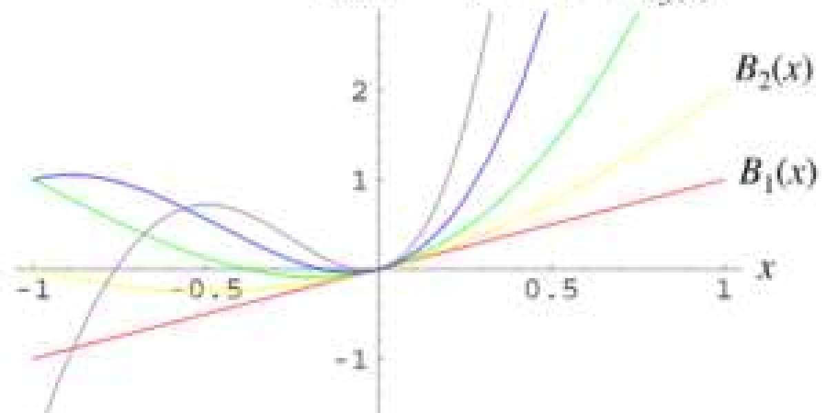
- Complete Bell Polynomials (Bₙ): Also known as "exponential" or "general" Bell polynomials, these are summations involving combinations. They're expressed as multi-variate polynomials.
- Partial Bell Polynomials (Bₙₖ): A subset of complete Bell polynomials that focus on particular groupings, making them especially useful for enumerative purposes, such as counting partitions of sets.
Both types showcase intricate relationships between combinations, partitions, and mathematical sequences.
The Mathematical Definition
To get a bit technical, Bell’s polynomials are defined as follows:
- Complete Bell Polynomials (Bₙ):
[latex]
B_n(x_1, x_2,..., x_n) = \sum_{k=1}^{n} B_{n,k}(x_1, x_2, ..., x_{n-k+1})
[/latex]
This formula represents the sum of all subsets of certain structures.
- Partial Bell Polynomials (Bₙₖ):
[latex]
B_{n,k}(x_1, x_2, ..., x_{n-k+1}) = \sum \frac{n!}{j₁! j₂!...j_{n-k}!} x_{n! j_1 x....
૪[/latex]
Understanding Bell’s Polynomials Made Simple
Bell’s polynomials are an essential concept in mathematics, especially in combinatorics and number theory. Though they might seem complex at first glance, their beauty lies in unraveling problems related to partitions and sequences. Whether you're a student trying to grasp the basics, a mathematician, or someone simply curious, this guide will break down Bell’s polynomials step by step so that you can understand their purpose, applications, and structure.
What Are Bell’s Polynomials?
At their core, Bell’s polynomials help in the process of studying partitions of numbers—how sets of numbers can be grouped or divided. Named after Eric Temple Bell, who made major contributions to mathematics, these polynomials are separated into two types:
- Partial Bell’s Polynomials
Partial Bell’s polynomials provide a way to study subsets and groupings of sequences. They're denoted as [latex]\( B_{n, k} \)[/latex], where [latex]\( n \)[/latex] represents a number's size, and \( k \) represents the number of partitions. Essentially, they show us how a number can be distributed across [latex]\( k \)[/latex] subsets.
For instance:
- If [latex]\( n = 3 \)[/latex] and [latex]\( k = 2 \)[/latex], the partial Bell’s polynomial will describe how three items can be grouped into two non-empty subsets.
- Complete Bell’s Polynomials
The complete Bell’s polynomial includes all potential partitions of a set. It’s represented as \( B_n \), which sums up all the [latex]\( B_{n, k} \)[/latex] terms where [latex]\( k \leq n \)[/latex]. It essentially calculates the total number of ways a number can be partitioned, making it highly relevant in combinatorics.
To summarize:
- Partial Bell’s Polynomials [latex](\( B_{n, k} \))[/latex] deal with specific partitions.
- Complete Bell’s Polynomials [latex](\( B_n \))[/latex] encompass all possible partitions.
Mathematical Formulation of Bell’s Polynomials
Bell’s polynomials may seem intimidating due to their notation, but they can be systematically understood. Here's how they’re represented:
Partial Bell’s Polynomial [latex](\( B_{n, k} \))[/latex]
This can be expressed as:
[latex]\[ B_{n,k}(x_1, x_2, ..., x_{n-k+1}) \][/latex]
This means it depends on [latex]\( n \)[/latex], the number of subsets, and [latex]\( x_i \)[/latex], a sequence of variables related to the group sizes.
Complete Bell’s Polynomial [latex](\( B_n \))[/latex]
The complete polynomial is a summation of all partial Bell polynomials:
[latex]\[ B_n(x_1, x_2, ..., x_n) = \sum_{k=1}^n B_{n,k}(x_1, x_2, ..., x_{n-k+1}) \][/latex]
If summations make you nervous, think of these as a way to lump together all possibilities for breaking [latex]\( n \)[/latex] into parts.
Key Applications of Bell’s Polynomials
Bell’s polynomials aren’t just abstract concepts—they solve real-world problems in fields such as statistics, physics, and computer science. Here’s where and how they’re used:
- Partitioning Problems
Bell’s polynomials are invaluable in problems requiring the division of a set into non-empty groups. For example, if you want to know how to distribute tasks among employees, Bell’s polynomials can be used to compute all the potential groupings.
- Combinatorics
Combinatorics, the study of counting and arrangements, heavily relies on Bell’s polynomials. They help determine the number of partitions of a set, which is fundamental in many counting-related problems.
- Moments in Statistics
Bell’s polynomials are used to calculate higher moments of random variables in probability and statistics. This is especially useful for deriving moments in cumulant expansions.
- Algorithms in Computer Science
Many sequence and combinatorial algorithms find Bell’s polynomials invaluable for developing efficiency and precision, specifically in recursive solutions.
- Physics and Mathematical Biology
These polynomials appear in studies of physical systems and biological growth models whenever partitioning structures are a core part of the equations.
Simple Example of Bell’s Polynomials in Action
Calculating Partial Bell’s Polynomial
Imagine we have [latex]\( n = 3 \)[/latex] and [latex]\( k = 2 \)[/latex], seeking to partition three elements into two groups. Using the partial Bell’s polynomial formula, we end up with:
[latex]\[ B_{3,2} = x_1x_2 + 3x_3 \][/latex]
This result shows how subsets of size 2 and 1 combine to form complete partitions.
Calculating Complete Bell’s Polynomial
Taking the same example [latex](\( n = 3 \))[/latex], the complete Bell’s polynomial sums all partial Bell’s polynomials:
[latex]\[ B_3 = B_{3,1} + B_{3,2} + B_{3,3} \][/latex]
This would yield the total number of ways to partition the set of 3 elements across all configurations.
How to Compute Bell’s Polynomials
While formulating Bell’s polynomials by hand is possible for small [latex]\( n \)[/latex], software tools like Mathematica, MATLAB, or programming languages such as Python can compute them more efficiently for larger values.
For example, in Python, libraries like SymPy allow computations of Bell’s polynomials with minimal code. Similarly, scientific tools like Wolfram Alpha offer built-in functions to calculate Bell numbers and polynomials.
Closing Thoughts on Bell’s Polynomials
Bell’s polynomials offer a fascinating interplay of structure and function, capturing the intricacy of partitions in a powerful mathematical framework. They simplify and formalize concepts underpinning everything from the study of set theory to machine learning algorithms.
Mastering Bell’s polynomials isn’t just about solving equations—it’s about unlocking a versatile tool applicable across industries. Start small, understand the basics, and explore their applications in real-world challenges.